Exercise 1 — Simulation of Adaptive Systems
This is a simulation exercise in FRTN15 Predictive Control. It should give you an introduction to adaptive control, in particular Model Reference Adaptive Systems (MRAS), see Figure 1.6 in the Textbook. The systems are modeled and simulated in the Matlab/Simulink environment. For those not familiar with Matlab/Simulink, this exercise will also serve as an opportunity to learn how to use it. Simulink will be used throughout the course, particularly in the hand-in assignments and the project, so it is important to become familiar with it as soon as possible.
This exercise involves building a Simulink model of a MRAS system and investigating its properties through simulation. Try to experiment with the parameters. The more you experiment and ask, the more you learn.
Before you start
Log in with you student account. Create a directory which will be used to store the files used in this exercise. Then navigate into the directory you just created.
Exercise 1.1
In this exercise we consider the problem of adapting a feed-forward gain. In order to perform the simulations, you will need to build a model of the system in Simulink. A library containing some per-defined elements is provided.
To download the zip file containing the .mdl and .m-files, press here. Unzip the file.The system looks like:
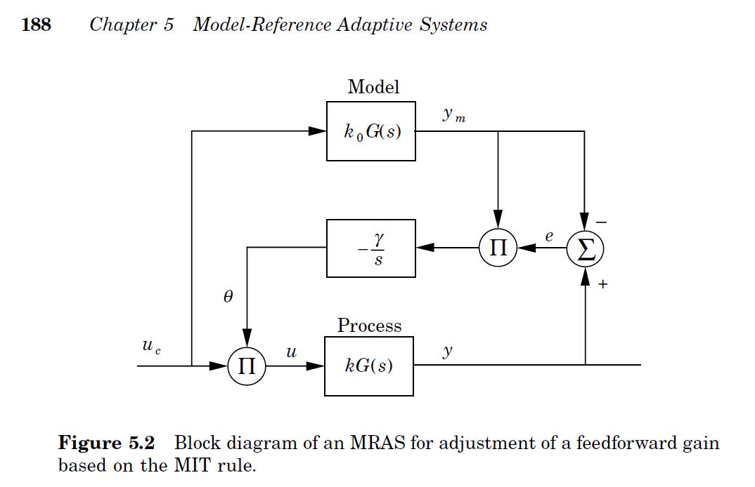
The objective is to find an update law, that adapts the feed-forward gain, θ (theta), so that the lower system behaves just like the upper reference system, see Figure 5.2 below.

Building the Mode
We first need to start Matlab. Write:
>matlab
When the Matlab prompt (which looks like >> ) has appeared, type into the Matlab command window:
>>ex11lib
to use the file ex11lib.mdl (which contains Simulink blocks for the first exercise). A new window will show up on the screen, containing the Simulink model.
The first task is to construct a Simulink model corresponding to the MRAS system in the first figure on this page. Begin by creating a new Simulink model:
-
Choose File/New/Model in the Simulink window
Now you can begin to construct the model. Use the predefined parts from the library ex11lib.mdl . Additional parts such as multiplication blocks, addition blocks and scopes (which are used to observe signals) can be found by typing
>>simulink
in the Matlab prompt. This opens a window with a graphical menu. For example, the scope block can be found under Sinks, and the multiplication and addition blocks can be found under Math Operations.
The library ex11lib.mdl contains transfer function blocks for the process and the model, as well as Subsystem blocks for the reference signal generator and adaption mechanism. Begin by dragging one of each of these blocks into your new Simulink window. Connect the system as shown in the above figure by clicking on the output port of on block, holding down the mouse button, and dragging the line to the input port of the next block. Note that you will need to use addition, multiplication, and scope blocks as well as the provided blocks.
Simulink Hints
If you want to change the parameters of a block (for example, change an addition block to a subtraction block, or change parameters in a transfer function), simply double click on the block. Similarly, double-clicking on a subsystem block opens another window displaying the contents of the subsystem. Double click on the reference generator block or the adaption mechanism block to see how they are constructed. (When changing parameters in the blocks from the library, namely the reference generator and adaption mechanism blocks, a window will appear with the message 'Attempt to change parameter of a block within a library link'. Simply click 'ok' and proceed as normal.)
Before running simulations with your model, you must specify both the adaption rate (gamma) and the reference offset (delta) in the Matlab environment. Write:
>>gamma = 1
>>delta = 1
in the Matlab prompt. Also, increase the simulation time from 10 senconds (the default) to 100 seconds by going to the 'Simulation/Simulation parameters' menu in your Simulink model and changing the stop time to 100.
Experiments
What parameter update law is used? To see this, double-click on the adjustment mechanism block and look at how the input signal (the output error) is processed.
Experiment with different offset levels on the reference signal (double click on the reference generator block and change the value of the offset block). What happens if the offset is chosen so that the reference signal always is negative?
Make the necessary modification for changing the update law to: (MIT-rule)
(Hint: Note that we now include the desired output ym in the update law. Replace the constant block in the adaption mechanism with another output port labeled 'ym' and proceed from there.)
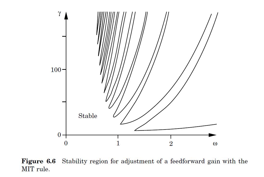
Change the reference signal so it becomes a sine wave with zero offset and use the second update strategy, i.e. the MIT-rule. (The library link for the adaption mechanism must be disabled in order to do this. Right click on the adaption mechanism block, select 'Link Options', and choose 'Disable Link') Study the system behavior for different values of the adaptation gain and the frequency of the reference signal. Set gamma to 20 and increase the reference signal's frequency to 0.3 Hz. Compare Figure below (taken from 6.6 on page 278 in 'Adaptive Control').
 Change the updating strategy to:
  (Lyapunov-rule)
This strategy is based on stability theory. Does it work better?
Exercise 1.2
In this exercise we will use Simulink to simulate Example 5.2 from the book [ Adaptive Control, page 190].
This example is summarized the pdf here. For this exercise, a model has already been built.
Begin by running the Matlab script ex12par.m. This initializes the parameters needed by the Simulink model. Type:
>>ex12par.m
in the Matlab prompt to run the script. Next, type:
>>ex12
to open the Simulink model. Try to identify the blocks in the diagram from Figure 1 in the pdf (or 5.4. on page 191 in the book).Now you are ready to start the simulation.
- Choose Simulation/Start or press Ctrl-t
Switch back to the Matlab main window (the one with the >> prompt), and modify the system's parameters which are given by a, b, am, bm, gamma where gamma stands for the adaptation rate.
Experiments
Try to reproduce figure 5.5, 5.6 and 5.7 in the example described in the pdf.How will the performance change with different values of the adaption rate?
Can you find any disadvantage with using a very fast adaption in this example?

