FRT041 System Identification, Hand-in problems 2017
Instructions:
FRTN35 System Identification course includes three mandatory hand-in problem sets, which should be solved individually. The problem sets are composed of exercises requiring analytic calculations as well as numerical calculations performed in Matlab or Julia. The purpose of the hand-in problem sets is to give You the opportunity to develop Your skills and get feedback from Your TA. The hand-in problem sets are also designed to help You prepare for the final exam and the course project.
Present Your results in a pdf report including well motivated answers to the problems stated in the problem text. Notice that the interpretation of Your results should be an integral part of the solution. Plots and hand-written calculations may be included as appendices and referred to in the solution text. Calculations should be clearly written and easy to follow. Number all equations for easy reference.
Hand-in problem 1
1.Compute the transfer function Y(z)/U(z) and the noise spectrum of the systemS: y(k) = 1.5y(k-1) -0.9y(k-2) + 0.4u(k-1) + w(k) + 0.7w(k-1)where {w(k)} is a zero-mean uncorrelated noise sequence with variance Var(w(k))=1. Include in your report a graphical spectral representation of the transfer function and the noise spectrum, also make sure you can differentiate between the concepts spectrum and bode diagram.2.Consider the continuous time signal y = sin(3*t)+10*sin(10*t).
- In Matlab or Julia, create a vector representing a sampled version of the signal with sampling interval t=0.1s. Use the commands fft/pwelch/periodogram to calculate the power spectrum of the sampled signal (in Julia, these are found in the package DSP.jl). Explain in a few words the relation between the function y and the characteristics of the spectrum. In particular, comment on location and magnitude of resonance peaks.
- Create a new vector representing the signal y sampled using the sampling interval t=0.5s. Again calculate and plot the power spectrum of the sampled signal using the command fft, pwelch, or similar. Explain the result. Does the spectrum look the way you expected?
3.(Optional:) Compute a one-step-ahead predictor for S. Compute the expected prediction error variance of your predictor.To be handed in to <FRTN35@list.control.lth.se>, deadline on September 16.
Hand-in problem 2
Exercise 6.1 in the textbook with the following modification:
S: y(k) + ay(k-1) = bu(k-1) + w(k) + cw(k-2)
Show that the parameter estimates will be biased. It should be clear from your solution that you have understood the problem well. Each step has to be motivated. Write clearly.
To be handed in to <FRTN35@list.control.lth.se>, deadline on September 30.
Hand-in problem 3
Consider the system
S: y(k) + ay(k-1) = bu(k-1) + w(k) + cw(k-2)
where {u(k)} and {w(k)} are zero mean white noise processes.
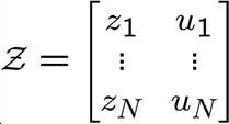
LSUse Matlab or Julia to compute an LS estimate of a and b, and the covariance matrix of the estimate. The regressor variables {u(k)} and {y(k)} are provided in downloadable files below. The number of observations is N=10000. Are the estimates consistent? IVUse Matlab or Julia to compute an estimate of a and b using the instrumental variable method. Also compute the covariance matrix of the estimate. Let {z(k)} where z(k)=az(k-1)+b u(k-1) where a and b are the LS estimates of a and b from above and the instrumental variable  Are the estimates consistent? Show this in a similar matter to how consistency was disproven for the LS-estimate in assignment 2. You may assume that the parameters a,b used to generate z are deterministic variables. PLRUse a pseudolinear regression method to estimate an ARMAX model. Note: there are several ways to perform pseudo-linear regression. One is detailed in example 6.6 in the book, another in section 11.4. They both share the commonality that they estimate the innovation/noise sequence for later use in the regressor.
You are supposed to implement the algorithms yourself, i.e. do not use the built-in Matlab commands in the System Identification Toolbox for this homework.
Time series data (Unix): data.mat
The file contains the variables u and y. They are loaded into the Matlab workspace with the command
>> load data
Time series data (Unix/Windows): u.txt , y.txt
The files contains the variables u and y. They are loaded into the Matlab workspace with the commands
>> load u.txt -ascii
>> load y.txt -ascii
Hand in code (.m-files, as code from pdfs is hard to run), numerical results, and computations. It should be clear from your solution that you have understood the problem well. Each step has to be motivated. Write clearly.
Hint: You may assume that w is uncorrelated ( E[ww^T]=s^2*I , where s^2=E[w^2]) when you compute the covariances of the estimates.
To be handed in to <FRTN35@list.control.lth.se>, deadline on October 7.
